Imagine handing someone three cards: dog, bites, and man.
You ask what happened. They cannot tell you. Did the dog bite the man, or did the man bite the dog? The words are all there. What is missing is their order.
We see that order immediately because we read from left to right. A Transformer needs a way to use it too. Its attention mechanism is excellent at comparing words and gathering relevant information. But the basic, unrestricted attention calculation does not come with a built-in idea of “first,” “before,” or “three places back.”
That is the problem positional encodings solve. They give the model information about where things are.
The interesting part is how that idea developed. The first approach sounds obvious: number the words. Then comes a better question: do we need the number, or do we need the distance between two words? Then comes a surprisingly elegant answer involving rotating arrows.
Let’s build those ideas one at a time. Each method now has a worked walkthrough: the same sentence, the same small embeddings, and the point where position changes the calculation. RoPE gets a longer two-clock example. You can follow the numbers without running code. Read the intuition first; the numbered steps make it concrete.
Start with attention: what should this word look at?
Consider this sentence:
The animal didn’t cross the street because it was tired.
To make sense of it, we look back at animal. The tired thing is probably the animal, not the street. Attention gives the model a way to make connections like this. Each word compares itself with other words, then gathers more information from the ones that seem useful.
Here is a picture of what we would like it to learn. The connections are illustrative, not measurements from a model.
But relevance is not just about meaning. In the red ball, “red” describes the word next to it. In a long paragraph, a nearby noun might be a better candidate than another noun several sentences away. Sometimes we need to look far back. Sometimes the word immediately before us matters most.
So the model needs both: what a word means and where it sits relative to other words.
A small vocabulary note: models actually work with tokens, which can be words, pieces of words, or punctuation. We’ll use whole words in the pictures so we can concentrate on the idea.
Our shared example: seven words, four numbers per word
We will use the same sentence for every walkthrough. The numbers are deliberately small, invented teaching values—not a trained model’s embeddings. Each word is one token in this example, and positions start at 0.
| Position | 0 | 1 | 2 | 3 | 4 | 5 | 6 |
|---|---|---|---|---|---|---|---|
| Word | the | cat | sat | on | the | soft | mat |
Notice the two copies of the. At the initial lookup, the same token gets the same embedding. Let’s see exactly where each design makes their journeys different.
| Position | Word | Embedding x · four numbers |
|---|---|---|
| 0 | the | (1.000, 0.000, 1.000, 0.000) |
| 1 | cat | (0.000, 1.000, 0.000, 1.000) |
| 2 | sat | (1.000, 1.000, 0.000, 0.000) |
| 3 | on | (0.000, 0.000, 1.000, 1.000) |
| 4 | the | (1.000, 0.000, 1.000, 0.000) |
| 5 | soft | (1.000, 0.000, 0.000, 1.000) |
| 6 | mat | (0.000, 1.000, 1.000, 0.000) |
Seven tokens give us a 7 × 4 embedding matrix. More generally, n tokens with d numbers each give n × d. The columns are learned coordinates, not named properties such as “animal” or “action.”
A small head we can follow without hiding the numbers
Real models learn weight matrices that make queries, keys, and values from each row. For this toy head we choose
especially simple matrices: queries and keys copy the input row; values reverse its four coordinates.
This is a legitimate choice of weights, but a deliberately simple one—not how trained weights usually look.
We write row vectors, so the convention is q = x W_Q, k = x W_K, v = x W_V.
| Word | q = k before position | v before position |
|---|---|---|
| the | (1.000, 0.000, 1.000, 0.000) | (0.000, 1.000, 0.000, 1.000) |
| cat | (0.000, 1.000, 0.000, 1.000) | (1.000, 0.000, 1.000, 0.000) |
| sat | (1.000, 1.000, 0.000, 0.000) | (0.000, 0.000, 1.000, 1.000) |
| on | (0.000, 0.000, 1.000, 1.000) | (1.000, 1.000, 0.000, 0.000) |
| soft | (1.000, 0.000, 0.000, 1.000) | (1.000, 0.000, 0.000, 1.000) |
| mat | (0.000, 1.000, 1.000, 0.000) | (0.000, 1.000, 1.000, 0.000) |
We will follow the second “the,” at position 4, when it looks backward. It may use positions 0 through 4; soft and mat are hidden because they are in the future. We apply this same causal mask to compare the designs, even though some of the original models also use attention that looks both ways.
To compare a query with a key, multiply corresponding coordinates and add. For example, “the” looking at “sat” gives
1×1 + 0×1 + 1×0 + 0×0 = 1. With four query/key coordinates, ordinary scaled attention divides this by
sqrt(4) = 2, giving a score of 0.5. DeBERTa’s three-term example below uses a different scale.
For n tokens, one head builds n query rows, n key rows, and n value rows. Comparing all queries with all keys makes an n × n score grid. We will display one row of that grid so we can see the arithmetic clearly.
The scores become attention weights through softmax: exponentiate the allowed scores, then divide each by their sum. Those weights mix the value rows, giving one updated row for each input token.
For reference, without any explicit position signal, the second “the” has the score row (1.000, 0.000, 0.500, 0.500, 1.000) for keys at positions 0–4. Both “the” keys tie. The causal mask itself provides some order structure, but there is no explicit distance signal in these matches.
The head output for this token is the weighted mixture of the five value rows: (0.272, 0.728, 0.272, 0.728).
This is one head’s output before an output projection, residual addition, normalization, or feed-forward block. Repeating the calculation for every query gives seven output rows, each with four numbers.
Now we can change one ingredient at a time. In the panels below, blue changes the input, amber changes relationships or scores, and purple changes query/key rotations. All calculations use full precision and are displayed rounded to three decimal places.
1. Give each word a seat number
Suppose you wanted to restore the order of our three cards. The simplest thing you could do is write a number on each one.
A Transformer does something similar, with one difference. It represents a word as a list of numbers, called an embedding. Instead of attaching a printed seat number, it adds another list of numbers describing that position. The model receives a mixture of the word information and the position information.
Learned absolute positions let training decide what each position’s list should be. Picture a drawer of seat labels: a label for the first token, another for the second, and so on. Models such as BERT and GPT-2 used this kind of position table. “Absolute” just means that a label describes a particular place in the sequence. The BERT paper describes its input embeddings, including position embeddings.
Worked example: learned positions
Step 0: Keep the sentence and choose a position table
Here is one possible toy table. We chose a tidy pattern so you can check the sums; a trained table need not follow any such pattern.
| Position | Word | Position row p | Input after adding: h = x + p |
|---|---|---|---|
| 0 | the | (0.000, 0.000, 0.000, 0.000) | (1.000, 0.000, 1.000, 0.000) |
| 1 | cat | (0.100, 0.000, 0.000, 0.050) | (0.100, 1.000, 0.000, 1.050) |
| 2 | sat | (0.200, 0.000, 0.000, 0.100) | (1.200, 1.000, 0.000, 0.100) |
| 3 | on | (0.300, 0.000, 0.000, 0.150) | (0.300, 0.000, 1.000, 1.150) |
| 4 | the | (0.400, 0.000, 0.000, 0.200) | (1.400, 0.000, 1.000, 0.200) |
| 5 | soft | (0.500, 0.000, 0.000, 0.250) | (1.500, 0.000, 0.000, 1.250) |
| 6 | mat | (0.600, 0.000, 0.000, 0.300) | (0.600, 1.000, 1.000, 0.300) |
Step 1: Compare the two copies of “the”
At position 0, (1.000, 0.000, 1.000, 0.000) + (0.000, 0.000, 0.000, 0.000) = (1.000, 0.000, 1.000, 0.000).
At position 4, (1.000, 0.000, 1.000, 0.000) + (0.400, 0.000, 0.000, 0.200) = (1.400, 0.000, 1.000, 0.200).
The lookup embeddings are identical. The rows entering attention are now different.
Step 2: Make queries, keys, and values from the combined rows
Our weights give q₄ = k₄ = (1.400, 0.000, 1.000, 0.200) and v₄ = (0.200, 1.000, 0.000, 1.400). Notice that values change too: they are made from the word-plus-position input, not the original word row.
Step 3: Follow one comparison
Against the first “the”: 1.4×1 + 0×0 + 1×1 + 0.2×0 = 2.4. Divide by 2 → 1.200. Against itself the dot is 1.4² + 1² + 0.2² = 3.0 → 1.500.
| Key position | Word | Query dot key | Scaled score |
|---|---|---|---|
| 0 | the | 2.400 | 1.200 |
| 1 | cat | 0.350 | 0.175 |
| 2 | sat | 1.700 | 0.850 |
| 3 | on | 1.650 | 0.825 |
| 4 | the | 3.000 | 1.500 |
Step 4: Convert scores to weights, then gather values
The two “the” connections no longer tie. This follows from the added position rows, not from a changed word identity.
The head output for this token is the weighted mixture of the five value rows: (0.368, 0.741, 0.259, 0.970).
This is one head’s output before an output projection, residual addition, normalization, or feed-forward block. Repeating the calculation for every query gives seven output rows, each with four numbers.
This gives the model a useful starting point. The word has an identity and a place.
But imagine that our drawer contains 512 labels. What happens when a document needs a 513th? There is no label waiting for it. Extending the table is possible, but the model has not automatically learned how to use those extra positions.
There is another question hiding here. “Red” can describe “ball” near the start of a sentence or near the end. Their seat numbers change, but being next to each other stays the same. Could our position system make that relationship easier to recognize?
Before we get there, let’s look at a clever alternative to a drawer of learned labels.
2. Use several clocks to describe a position
Think about the hands on a clock. The second hand moves quickly. The minute hand moves more slowly. The hour hand moves more slowly still. Together, they describe the time more fully than any one hand could.
Now imagine a collection of clock hands that advances every time we move one token along a sentence. One hand takes a large step. Another takes a small step. Another barely moves. A position is described by the collection of angles.
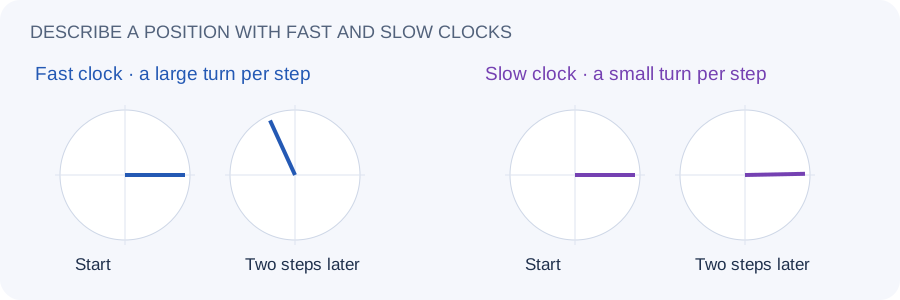
Why more than one clock? A single hand eventually comes around again. Looking at the minute hand alone, you cannot tell which hour it is. Having hands that turn at different speeds gives the model a richer pattern for each position.
The original 2017 Transformer used sine and cosine functions to make these patterns. That is where the name sinusoidal positional encoding comes from. You can think of those functions as a way to write down a clock hand’s position using two numbers. The resulting numbers are added to the word embedding, just like the seat labels. Attention Is All You Need introduced this design alongside a learned-position alternative.
Worked example: sinusoidal positions
Step 0: Make two clock pairs
For four dimensions and base 10,000, the row is (sin m, cos m, sin(0.01m), cos(0.01m)). Angles here are in radians. The first pair changes quickly; the second changes slowly.
| Position | Word | Clock row | Input after adding |
|---|---|---|---|
| 0 | the | (0.000, 1.000, 0.000, 1.000) | (1.000, 1.000, 1.000, 1.000) |
| 1 | cat | (0.841, 0.540, 0.010, 1.000) | (0.841, 1.540, 0.010, 2.000) |
| 2 | sat | (0.909, -0.416, 0.020, 1.000) | (1.909, 0.584, 0.020, 1.000) |
| 3 | on | (0.141, -0.990, 0.030, 1.000) | (0.141, -0.990, 1.030, 2.000) |
| 4 | the | (-0.757, -0.654, 0.040, 0.999) | (0.243, -0.654, 1.040, 0.999) |
| 5 | soft | (-0.959, 0.284, 0.050, 0.999) | (0.041, 0.284, 0.050, 1.999) |
| 6 | mat | (-0.279, 0.960, 0.060, 0.998) | (-0.279, 1.960, 1.060, 0.998) |
Step 1: Follow the second “the”
At position 4, its original row (1.000, 0.000, 1.000, 0.000) receives clock row (-0.757, -0.654, 0.040, 0.999), producing (0.243, -0.654, 1.040, 0.999). The first “the” instead receives (0.000, 1.000, 0.000, 1.000). Same word, different clock reading.
Step 2: Make q, k, and v after the addition
q₄ = k₄ = (0.243, -0.654, 1.040, 0.999); v₄ = (0.999, 1.040, -0.654, 0.243). This is the same place in the pipeline as learned absolute positions. Only the source of the added position row changed.
Step 3: Multiply corresponding coordinates and add
For the first “the,” k₀ = (1.000, 1.000, 1.000, 1.000). The raw match is (0.243×1) + (-0.654×1) + (1.040×1) + (0.999×1) ≈ 1.629. Divide by 2 → 0.814.
| Key position | Word | Raw match | Scaled score |
|---|---|---|---|
| 0 | the | 1.629 | 0.814 |
| 1 | cat | 1.207 | 0.603 |
| 2 | sat | 1.103 | 0.551 |
| 3 | on | 3.751 | 1.875 |
| 4 | the | 2.566 | 1.283 |
Step 4: Gather the changed value rows
These clock patterns influence both the matches and the values, because both were made after the input addition.
The head output for this token is the weighted mixture of the five value rows: (1.523, 0.801, -0.171, 0.558).
This is one head’s output before an output projection, residual addition, normalization, or feed-forward block. Repeating the calculation for every query gives seven output rows, each with four numbers.
The pleasant thing is that a formula can keep producing patterns beyond the positions in a fixed table. We do not run out of labels in the same way.
Still, being able to produce a label is different from the model knowing what to do with it. A model trained on short passages can struggle with the patterns and relationships in much longer ones. And we are still handing it a description of each individual position, then asking it to work out the relationship between two positions.
Let’s make that relationship explicit.
3. Describe how far apart the words are
Read these two phrases:
- the red ball
- after a surprisingly long afternoon, the red ball
“Red” moved. “Ball” moved. But “red” is still immediately before “ball.” That feels like the useful fact, doesn’t it?
This is the idea behind relative positions. Instead of telling each word only “you are in seat 9,” we give its interactions information such as “this word is one step ahead” or “that word is three steps behind.”
Notice where the information is useful. When “red” considers “ball,” attention is already asking whether they belong together. We can bring their relative position into that very comparison.
Shaw: learn what “one step away” means
In 2018, Shaw and colleagues introduced learned representations for relative offsets. Think of little relationship labels: one before, two before, one after. The same label can be used anywhere in a sentence. The model can learn what to do with it rather than learning separate versions of the relationship at every pair of seat numbers.
To keep the collection manageable, distant offsets share labels beyond a chosen cutoff. That saves space, but it also means some far-apart relationships become indistinguishable to the position system. Their method brings relative information into both the matching and the information gathered. Self-Attention with Relative Position Representations.
Worked example: Shaw relative representations
Step 0: Use relationship labels instead of seat labels
Our gap is query position minus key position: a positive gap means the key is earlier. This reverses the original paper’s indexing convention, so we relabel the learned table consistently. Clip gaps to −2…2.
| Gap label | Relative-key row | Relative-value row |
|---|---|---|
| -2 | (-0.200, 0.000, 0.000, 0.000) | (0.000, -0.100, 0.000, 0.000) |
| -1 | (-0.100, 0.000, 0.000, 0.000) | (0.000, -0.050, 0.000, 0.000) |
| 0 | (0.000, 0.000, 0.000, 0.000) | (0.000, 0.000, 0.000, 0.000) |
| 1 | (0.100, 0.000, 0.000, 0.000) | (0.000, 0.050, 0.000, 0.000) |
| 2 | (0.200, 0.000, 0.000, 0.000) | (0.000, 0.100, 0.000, 0.000) |
Step 1: Follow “the” looking at “cat”
The query is at 4 and the key is at 1. Gap 3 is clipped to 2. For this pair, add (0.2, 0, 0, 0) to cat’s key (0, 1, 0, 1) → (0.2, 1, 0, 1). The stored cat key has not permanently changed; the extra row belongs to this particular relationship.
Step 2: Score the relationship
The query (1, 0, 1, 0) dotted with (0.2, 1, 0, 1) gives 0.2. Divide by 2 → 0.100, rather than the content-only score 0.
| Key | Gap → clipped gap | Content-only score | Score with relative key |
|---|---|---|---|
| 0: the | 4 → 2 | 1.000 | 1.100 |
| 1: cat | 3 → 2 | 0.000 | 0.100 |
| 2: sat | 2 → 2 | 0.500 | 0.600 |
| 3: on | 1 → 1 | 0.500 | 0.550 |
| 4: the | 0 → 0 | 1.000 | 1.000 |
Step 3: Change what is gathered as well
Cat’s value is (1, 0, 1, 0). For this gap we add (0, 0.1, 0, 0) → (1, 0.1, 1, 0). Thus the weighted mixture carries relationship information as well as content.
Step 4: Mix the pair-specific values
Offsets beyond the clipping limit share a label. This head can distinguish “nearby” and “farther away,” but its position table treats gaps 2, 3, and 4 alike.
The head output for this token is the weighted mixture of the five value rows: (0.273, 0.784, 0.282, 0.727).
This is one head’s output before an output projection, residual addition, normalization, or feed-forward block. Repeating the calculation for every query gives seven output rows, each with four numbers.
Transformer-XL: keep the relationship when you turn the page
Now imagine reading a book one page at a time. You want the next page to use what you learned on the previous one. But if both pages start their numbering at 1, the old seat numbers become confusing.
Transformer-XL reused representations from earlier text segments. Relative positions helped it describe how far those remembered tokens were from the current tokens, across segment boundaries. The important development was that position had to work with a continuing memory, not just within one isolated passage. Transformer-XL, 2019.
Worked example: Transformer-XL across a segment boundary
Step 0: Split our sentence into memory and current text
Remember positions 0–1 (“the cat”) from the previous segment. Process positions 2–6 (“sat on the soft mat”) now. For this first-layer toy, pretend the stored rows equal the listed token rows; real memory contains earlier hidden representations.
Step 1: Count the rows
The current segment has 5 query rows. Together, memory and current text supply 7 key and value rows, making a 5 × 7 score grid before masking. Following global position 4 gives access to keys 0–4, including the remembered “the cat.”
Step 2: Describe distance across the boundary
For the current “the” at global 4 and remembered “cat” at global 1, gap = 3. Use relative clock row (0.141, -0.990, 0.030, 1.000). Their segment-local numbers need not be compared as if they were positions in one isolated segment.
Step 3: Combine four kinds of match
In this simplified attention calculation, the content projections and relative-position projection are identities. Use learned-bias examples u = (0.1, 0, 0, 0) and b = (0, 0.1, 0, 0). The raw score is q·k + q·R(gap) + u·k + b·R(gap). These are a content match, a content–distance match, a content preference, and a distance preference. Divide their sum by 2.
| Key | q·k | q·R | u·k | b·R | Scaled total |
|---|---|---|---|---|---|
| 0: the | 2.000 | -0.717 | 0.100 | -0.065 | 0.659 |
| 1: cat | 0.000 | 0.171 | 0.000 | -0.099 | 0.036 |
| 2: sat | 1.000 | 0.929 | 0.100 | -0.042 | 0.994 |
| 3: on | 1.000 | 0.851 | 0.000 | 0.054 | 0.953 |
| 4: the | 2.000 | 0.000 | 0.100 | 0.100 | 1.100 |
Step 4: Gather from memory and current values
Memory extends the set of keys and values; it does not create new output rows for the old segment.
The head output for this token is the weighted mixture of the five value rows: (0.322, 0.668, 0.332, 0.678).
This is one head’s output before an output projection, residual addition, normalization, or feed-forward block. Repeating this for the five current queries gives five current output rows, each with four numbers. The two memory rows are consulted, not emitted again.
T5: we may not need a separate label for every distance
When giving directions, we often say “next door,” “a few houses away,” or “across town.” We are precise nearby and less precise far away.
T5 takes a similar approach. Nearby distances get fine distinctions. Larger distances are grouped into wider buckets. For each bucket, an attention head learns a number that nudges a connection’s score up or down.
Different heads can learn different distance preferences: one might often look nearby, while another pays more attention farther back. These are preferences, not rules about which words must connect. T5, first released in 2019.
Worked example: T5 distance buckets
Step 0: Choose a small learned bias table
This is an invented table for one head, not T5’s real bucket boundaries or trained values. Direction is “backward” because our comparison uses causal attention.
| Distance bucket | Learned score adjustment |
|---|---|
| self | 0.000 |
| one back | 0.300 |
| two back | 0.100 |
| 3–4 back | -0.200 |
| 5+ back | -0.400 |
Step 1: Keep q, k, and v as they were
For the second “the,” q₄ = (1, 0, 1, 0). Its content-only score row is (1, 0, 0.5, 0.5, 1). We have not added a position vector to any word row.
Step 2: Look up one bias for each pair
Looking from position 4 to “on” at 3 gives gap 1. Content score 0.5, bucket bias +0.3, new score 0.8. Looking back to the first “the” gives gap 4: 1.0 − 0.2 = 0.8.
| Key | Gap | Bucket | Content score | Add bias | New score |
|---|---|---|---|---|---|
| 0: the | 4 | 3–4 back | 1.000 | -0.200 | 0.800 |
| 1: cat | 3 | 3–4 back | 0.000 | -0.200 | -0.200 |
| 2: sat | 2 | two back | 0.500 | 0.100 | 0.600 |
| 3: on | 1 | one back | 0.500 | 0.300 | 0.800 |
| 4: the | 0 | self | 1.000 | 0.000 | 1.000 |
Step 3: Gather values with the new weights
The score row changed. The query, key, and value rows did not receive any direct positional transformation in this calculation.
The head output for this token is the weighted mixture of the five value rows: (0.310, 0.731, 0.269, 0.690).
This is one head’s output before an output projection, residual addition, normalization, or feed-forward block. Repeating the calculation for every query gives seven output rows, each with four numbers.
DeBERTa: keep meaning and position separate while comparing
Earlier, we mixed the seat label into the word embedding. DeBERTa asks whether we can keep the two descriptions separate for longer.
Imagine two cards for each token: one describes its content; the other helps describe relative position. Attention can then consider content-to-content matches and how content relates to position, instead of starting from one blended description. That separation is the intuition behind disentangled attention. DeBERTa, 2020.
Worked example: DeBERTa’s separate comparisons
Step 0: Give content and position their own representations
For the toy, content projections and the position-key projection are identities. The position-query projection halves the first coordinate and copies the other three. For a signed offset g, the relative-position row is P(g) = (0.1g, 0.2, 0, 0). Actual position rows and projections are learned; this formula just specifies our invented table.
Step 1: Match the content
“The” at 4 looking at “cat” at 1: content query (1, 0, 1, 0) meets content key (0, 1, 0, 1) → content–content match 0.
Step 2: Add two directional position matches
Gap = 3. The content query meets position key P(+3) = (0.3, 0.2, 0, 0) → 0.3. Project P(−3) to position query (−0.15, 0.2, 0, 0) meets cat’s content key → 0.2. Both directions participate, using opposite signed offsets.
Step 3: Combine the three matches
For cat, raw total 0 + 0.3 + 0.2 = 0.5. For this three-term, four-coordinate example, divide by sqrt(3×4) ≈ 3.464 → 0.144. We use the three-term attention scale rather than quietly treating it as a single dot product.
| Key | Content↔content | Content→position | Position→content | Scaled total |
|---|---|---|---|---|
| 0: the | 2.000 | 0.400 | -0.200 | 0.635 |
| 1: cat | 0.000 | 0.300 | 0.200 | 0.144 |
| 2: sat | 1.000 | 0.200 | 0.100 | 0.375 |
| 3: on | 1.000 | 0.100 | 0.000 | 0.318 |
| 4: the | 2.000 | 0.000 | 0.000 | 0.577 |
Step 4: Gather content values
Relative-position representations affected the score through separate matches. They were not blended into each initial token row.
The head output for this token is the weighted mixture of the five value rows: (0.330, 0.659, 0.341, 0.670).
This is one head’s output before an output projection, residual addition, normalization, or feed-forward block. Repeating the calculation for every query gives seven output rows, each with four numbers.
These developments are related ideas, not a ladder where every new method makes the previous one obsolete. Now let’s try a distance preference that does not need to be learned at all.
4. Let distance nudge attention: ALiBi
Suppose you are reading a paragraph and encounter “it.” Usually, you start looking for its referent nearby. You can look farther back, but you need a good reason.
ALiBi gives attention that sort of preference. A token farther in the past pays a larger distance penalty when its attention score is calculated. If two candidates have equally good content matches, the closer one wins.
Different heads pay different rates. Some have a strong preference for nearby tokens; others have a gentler penalty and can look farther back more easily. These rates are fixed rather than learned.
Why is this useful for longer text? “Charge a little more for each extra step” still makes sense at distances we did not see during training. There is no new seat label to invent. ALiBi demonstrated better length extrapolation in its experiments. The tradeoff is that a useful detail buried far back also has to overcome that distance cost. Train Short, Test Long, 2021.
Worked example: ALiBi
Step 0: Choose a rate for this head
Use a fixed 0.25 per token step. This is a teaching rate; real ALiBi assigns a prescribed set of rates across heads.
Step 1: Compute the content matches first
The second “the” has q₄ = (1, 0, 1, 0). Before distance penalties, the score row is (1, 0, 0.5, 0.5, 1). Keys and values remain as listed in the shared setup.
Step 2: Subtract the price of distance
For the first “the,” gap 4 costs 0.25×4 = 1. Its score changes from 1 to 0. For “on,” gap 1 costs 0.25; its score changes from 0.5 to 0.25.
| Key | Gap | Content score | Distance penalty | New score |
|---|---|---|---|---|
| 0: the | 4 | 1.000 | -1.000 | 0.000 |
| 1: cat | 3 | 0.000 | -0.750 | -0.750 |
| 2: sat | 2 | 0.500 | -0.500 | 0.000 |
| 3: on | 1 | 0.500 | -0.250 | 0.250 |
| 4: the | 0 | 1.000 | 0.000 | 1.000 |
Step 3: Mix values according to the new weights
The identical “the” keys now receive different weights because one is four steps away and the other is at the query’s own position. A distant key could still win if its content match were strong enough.
The head output for this token is the weighted mixture of the five value rows: (0.271, 0.773, 0.227, 0.729).
This is one head’s output before an output projection, residual addition, normalization, or feed-forward block. Repeating the calculation for every query gives seven output rows, each with four numbers.
So far we have given tokens labels and given connections distance preferences. Next, we change the way the comparison is represented.
5. Turn position into a rotation: RoPE
Hold out two pencils so they point in the same direction. Now turn one a little. They are less aligned. Turn it farther, and their alignment changes again.
Now keep the angle between them fixed and turn both together. They still have the same alignment. You have changed the direction each pencil points, but not their relationship.
That simple observation is the heart of Rotary Position Embedding, or RoPE.
To connect it to attention, we need just two names. A query describes what a token is looking for. A key describes what another token offers for matching. Both are lists of numbers learned by the model. Attention compares them to decide how much information to gather from that token.
Imagine a tiny part of each query and key as an arrow on a flat sheet of paper. RoPE turns those arrows by an amount determined by their token positions before comparing them. The comparison can then use both the original content and the relative turn. RoFormer, 2021.
RoPE with d = 4 and seven words, fully worked
Step 0: Locate the change in the pipeline
The input embedding row is not directly modified by RoPE. Neither is v. The positional turn happens to q and k just before their dot product. Later token representations still change, because the resulting attention weights gather different information.
Step 1: Follow the two copies of “the”
At positions 0 and 4, their lookup rows are both (1, 0, 1, 0). With our chosen first-layer weights, both also have q = k = (1, 0, 1, 0) and v = (0, 1, 0, 1) before rotation. In later layers, their different contexts can already give them different content rows.
Step 2: Split each matching row into two arrows
Cut (1, 0, 1, 0) into pair A = (1, 0) and pair B = (1, 0). Each pair is an arrow in its own flat plane. Four coordinates make two pairs; 128 coordinates make 64 pairs.
(1, 0) → fast arrow Pair B · coordinates 2–3
(1, 0) → slow arrow
Step 3: Give the arrows different speeds
Use 90° per position for pair A and 10° per position for pair B. These are deliberately simple teaching speeds. Standard d = 4 RoPE with base 10,000 uses 1 radian and 0.01 radian per position instead.
| Position | Word | Pair A angle | Pair B angle |
|---|---|---|---|
| 0 | the | 0° | 0° |
| 1 | cat | 90° | 10° |
| 2 | sat | 180° | 20° |
| 3 | on | 270° | 30° |
| 4 | the | 360° (same direction as 0°) | 40° |
| 5 | soft | 450° (same direction as 90°) | 50° |
| 6 | mat | 540° (same direction as 180°) | 60° |
Step 4: Turn an arrow, then rejoin the pairs
An arrow starting at (1, 0) becomes (cos φ, sin φ) after a turn of φ. First hold the starting content fixed and see what happens if this same “the” row occupies each possible position. This is a position-only demonstration, not a claim that every word has the same vector.
| Position | Fast pair A | Slow pair B | Rejoined “the” row |
|---|---|---|---|
| 0 | (1.000, 0.000) | (1.000, 0.000) | (1.000, 0.000, 1.000, 0.000) |
| 1 | (0.000, 1.000) | (0.985, 0.174) | (0.000, 1.000, 0.985, 0.174) |
| 2 | (-1.000, 0.000) | (0.940, 0.342) | (-1.000, 0.000, 0.940, 0.342) |
| 3 | (0.000, -1.000) | (0.866, 0.500) | (0.000, -1.000, 0.866, 0.500) |
| 4 | (1.000, 0.000) | (0.766, 0.643) | (1.000, 0.000, 0.766, 0.643) |
| 5 | (0.000, 1.000) | (0.643, 0.766) | (0.000, 1.000, 0.643, 0.766) |
| 6 | (-1.000, 0.000) | (0.500, 0.866) | (-1.000, 0.000, 0.500, 0.866) |
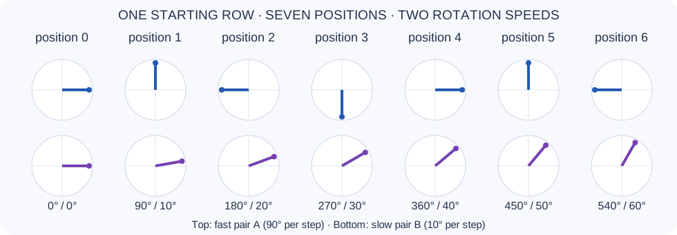
The actual “the” rows are now (1, 0, 1, 0) at 0 and (1, 0, 0.766, 0.643) at 4. The first pair alone repeats every four steps in this toy. The second pair separates those positions. Multiple speeds reduce this ambiguity over useful ranges; they do not promise an unlimited, unique distance code.
Step 5: Check equal gaps while keeping content fixed
Temporarily give the compared query and key the same starting vector (1, 0, 1, 0). We are isolating position, so these are not the actual “on/cat” and “mat/the” content pairs from our sentence.
Case 1: query at 3, key at 1, gap = 2.
q = (0.000, -1.000, 0.866, 0.500), k = (0.000, 1.000, 0.985, 0.174).
Fast-pair contribution -1.000 + slow-pair contribution 0.940 = raw dot product -0.060.
Case 2: query at 6, key at 4, gap = 2.
q = (-1.000, 0.000, 0.500, 0.866), k = (1.000, 0.000, 0.766, 0.643).
Fast-pair contribution -1.000 + slow-pair contribution 0.940 = raw dot product -0.060.
Both raw dots are −0.060 to three decimals. Scaled attention divides by 2, giving about −0.030, before masking and softmax. The raw dot and the scaled score are different stages of the pipeline.
Step 6: See the shortcut for identical starting arrows
Each pair contributes cos(speed × gap), so the raw dot is cos(90°×gap) + cos(10°×gap). This shortcut applies to our chosen identical unit arrows; general queries and keys also bring their starting content into the match.
| Gap | Fast pair | Slow pair | Raw dot |
|---|---|---|---|
| 0 | 1.000 | 1.000 | 2.000 |
| 1 | 0.000 | 0.985 | 0.985 |
| 2 | -1.000 | 0.940 | -0.060 |
| 3 | 0.000 | 0.866 | 0.866 |
| 4 | 1.000 | 0.766 | 1.766 |
| 5 | 0.000 | 0.643 | 0.643 |
| 6 | -1.000 | 0.500 | -0.500 |
Step 7: Change the content and observe direction
Keep q = (1, 0, 1, 0) but choose k = (0, 1, 0, 1). The raw dot now follows sin(90°×gap) + sin(10°×gap), with gap = query position minus key position.
| Gap | Raw dot for these different starting rows |
|---|---|
| 0 | 0.000 |
| 1 | 1.174 |
| 2 | 0.342 |
| -1 | -1.174 |
Now +1 gives 1.174, while −1 gives −1.174. In this example the match distinguishes which side the key is on. A causal mask will still forbid future keys; these dots alone are not permission to attend to them.
Step 8: Return to the actual seven-word sentence
Now use each word’s own starting row from the shared table. The position-only shortcut no longer applies to every pair. Rotate each q and k using its actual position; keep v unchanged.
| Position | Word | Actual rotated q = rotated k | Unrotated v |
|---|---|---|---|
| 0 | the | (1.000, 0.000, 1.000, 0.000) | (0.000, 1.000, 0.000, 1.000) |
| 1 | cat | (-1.000, 0.000, -0.174, 0.985) | (1.000, 0.000, 1.000, 0.000) |
| 2 | sat | (-1.000, -1.000, 0.000, 0.000) | (0.000, 0.000, 1.000, 1.000) |
| 3 | on | (0.000, 0.000, 0.366, 1.366) | (1.000, 1.000, 0.000, 0.000) |
| 4 | the | (1.000, 0.000, 0.766, 0.643) | (0.000, 1.000, 0.000, 1.000) |
| 5 | soft | (0.000, 1.000, -0.766, 0.643) | (1.000, 0.000, 0.000, 1.000) |
| 6 | mat | (0.000, -1.000, 0.500, 0.866) | (0.000, 1.000, 1.000, 0.000) |
For the second “the,” q̂₄ = (1, 0, 0.766, 0.643). Against “cat” at 1, k̂₁ = (−1, 0, −0.174, 0.985). The raw dot is −1 + (0.766×−0.174) + (0.643×0.985) ≈ −0.500; scaled score −0.250. This is content and position working together.
| Key position | Word | Raw dot after rotation | Scaled score |
|---|---|---|---|
| 0 | the | 1.766 | 0.883 |
| 1 | cat | -0.500 | -0.250 |
| 2 | sat | -1.000 | -0.500 |
| 3 | on | 1.158 | 0.579 |
| 4 | the | 2.000 | 1.000 |
Step 9: Convert scores to weights and gather the original values
The two “the” embeddings stayed the same at lookup. Their rotated keys changed the comparisons, which changes what the current token gathers.
The head output for this token is the weighted mixture of the five value rows: (0.309, 0.833, 0.167, 0.691).
This is one head’s output before an output projection, residual addition, normalization, or feed-forward block. Repeating the calculation for every query gives seven output rows, each with four numbers.
The picture to keep: two stacked turntables, one fast and one slow. Each token places its content arrows on them. Position turns the tables. Attention compares a query’s arrows with a key’s arrows; shifting both by the same amount preserves their relative turns when their starting content is held fixed.
Optional: why does the absolute position cancel?
Rotations preserve dot products. Turn q by mθ and k by nθ; undo the same mθ turn on both. You are left comparing q with k turned by (n−m)θ. The starting vectors still determine the content part of the match. In complex-number notation, the same cancellation comes from multiplying one rotated pair by the conjugate of the other.
Why many arrows, rather than just two?
Remember the fast and slow clocks? RoPE uses that same idea of several rotation speeds. Different pairs of numbers in a query or key turn at different rates. Fast turns give detailed changes over nearby positions. Slower turns give a more gradual signal over longer distances.
There is an important difference from the earlier sinusoidal method. There, clock readings were added to the word’s representation. Here, they control how the query and key are turned before a match.
Add a clock reading
The word starts its journey carrying meaning mixed with a position pattern.
Turn the matching arrows
Position changes the comparison used to decide where attention should look.
The information being gathered, called the value, is not rotated by standard RoPE. A useful way to picture it: we adjust the way we choose a book from the shelf, rather than turning all the writing inside the book.
One thing to be careful about: RoPE is not a rule that says “nearby words always match better.” Our equal-gap demonstration fixes the starting arrows to make the geometry visible. Real queries and keys differ with content, and many rotating pairs contribute together. The model learns how to use that positional structure.
6. What happens when the document gets longer?
We have a method that describes relative relationships. Surely we can now read a document of any length?
There is a catch. The model learned from documents of certain lengths. A much longer document produces combinations of clock angles and distances that may be unfamiliar, especially for slowly turning pairs. Having a position system that accepts a large number does not guarantee that the model will use it well.
Imagine practising with a ruler marked from 0 to 4, then being handed one that runs to 16. You can read the numbers, but the patterns you learned on the short ruler may not transfer smoothly.
Position Interpolation: squeeze the longer ruler into the familiar span
One approach is to compress the position scale. To fit four times as many tokens into the old range, we treat position 12,000 like position 3,000 for the rotations.
This helps keep the rotation range familiar. The cost is that nearby positions also become more similar: we squeezed the small gaps as well as the large ones. Models can be fine-tuned to adapt to the new scale. Position Interpolation, 2023.
NTK-aware scaling and YaRN: don’t slow every clock equally
If the fast clocks help distinguish neighbours, perhaps we should preserve more of their detail while slowing the clocks that describe longer stretches.
NTK-aware scaling changes the spacing of rotation speeds, stretching the slower ones more while leaving the fastest unchanged. YaRN makes a more explicit distinction: keep fast rotations, slow down slow rotations, and blend the treatment in between. It also adjusts the attention score scale.
Slow every clock
Simple compression, including the clocks that distinguish neighbours.
Stretch speeds unevenly
Preserve the fastest rotation while slowing longer-range ones more.
Treat fast and slow differently
Keep fast clocks, slow slow clocks, and blend the middle.
The aim is to gain room for long documents without losing so much detail between neighbouring tokens. YaRN, 2023, develops this frequency-selective approach.
Other approaches, such as LongRoPE, search for different stretching factors across the rotating pairs. LongRoPE develops that search-based approach. A larger RoPE base also makes the slower clocks turn more slowly. These are ways of reshaping the position scale, not promises that every distant detail will be retrieved correctly.
Where does this change our rows? All three keep the same token embeddings and the same query/key/value pipeline as RoPE. They change the schedule of turns applied to the query and key pairs. Interpolation compresses positions uniformly; NTK-aware scaling and YaRN treat rotation speeds differently. The word rows do not get longer, and no extra word rows are created.
Worked examples: extending the same four-number head
For this section we switch from the 90°/10° teaching clocks to standard d = 4 RoPE rates: 1 and 0.01 radians per position. The sentence, word embeddings, and weight matrices remain the same. Assume a training window of 4,096 tokens and a desired 4× extension. The seven words let us inspect the changed arithmetic; they do not demonstrate long-context quality.
| Recipe | Fast pair · radians/step | Slow pair · radians/step | Position 4 · fast / slow angles |
|---|---|---|---|
| Unextended standard RoPE | 1.000 | 0.010000 | 4.000 / 0.040000 rad |
| Position Interpolation | 0.250 | 0.002500 | 1.000 / 0.010000 rad |
| NTK-aware | 1.000 | 0.002500 | 4.000 / 0.010000 rad |
| YaRN | 1.000 | 0.003835 | 4.000 / 0.015341 rad |
| Example LongRoPE candidate | 0.500 | 0.002500 | 2.000 / 0.010000 rad |
Position Interpolation
Step 0: Compress the position scale
Position m becomes m/4. Equivalently, divide both rotation rates by 4: 1 → 0.25 and 0.01 → 0.0025. Position 4 takes the old position-1 angles.
Step 1: Turn the second “the” with the revised rates
Its pre-rotation query is still (1, 0, 1, 0). The revised rotation gives (0.540, 0.841, 1.000, 0.010). Each key receives its corresponding turn. The value rows stay as listed in the shared setup.
Step 2: Compute matches and mix values
Compare that query with the revised keys, divide raw dots by 2, then turn the scores into weights.
| Key | 0: the | 1: cat | 2: sat | 3: on | 4: the |
|---|---|---|---|---|---|
| Scaled score | 0.770 | 0.345 | 0.679 | 0.501 | 1.000 |
| Attention weight | 21.8% | 14.2% | 19.9% | 16.7% | 27.4% |
The second “the” gathers the original value rows into head output (0.309, 0.659, 0.341, 0.691). Embeddings and values were not directly changed by the positional rule. The seven query rows still produce seven output rows.
NTK-aware
Step 0: Change the base rather than every position
For the usual base-change rule with d = 4 and scale 4, the new base is 10,000 × 4^(4/(4−2)) = 160,000. Its rates are 1 and 1/sqrt(160,000) = 0.0025. The fastest rate stays put; the slower one changes.
Step 1: Turn the second “the” with the revised rates
Its pre-rotation query is still (1, 0, 1, 0). The revised rotation gives (-0.654, -0.757, 1.000, 0.010). Each key receives its corresponding turn. The value rows stay as listed in the shared setup.
Step 2: Compute matches and mix values
Compare that query with the revised keys, divide raw dots by 2, then turn the scores into weights.
| Key | 0: the | 1: cat | 2: sat | 3: on | 4: the |
|---|---|---|---|---|---|
| Scaled score | 0.173 | 0.074 | 0.247 | 0.501 | 1.000 |
| Attention weight | 15.0% | 13.6% | 16.2% | 20.9% | 34.3% |
The second “the” gathers the original value rows into head output (0.345, 0.702, 0.298, 0.655). Embeddings and values were not directly changed by the positional rule. The seven query rows still produce seven output rows.
YaRN
Step 0: Classify the two clocks by training-window rotations
The fast clock made about 651.9 turns in 4,096 positions; the slow one made about 6.52. Using YaRN’s conventional blend thresholds of 1 and 32 turns, the fast pair is preserved. The slow pair falls in the blend region, not the fully compressed region.
Step 1: Blend the slow rate and apply the attention-scale correction
The slow pair’s blend weight is (6.52 − 1) / (32 − 1) ≈ 0.178. Blend rate 0.01 with rate 0.0025 → 0.003835. The conventional attention correction multiplies q and k by 1 + 0.1 ln(4) ≈ 1.139, multiplying dot-product scores by about 1.296. We include that correction below. A four-coordinate head has no other pairs; a wide head has many intermediate cases.
Step 2: Turn the second “the” with the revised rates
Its pre-rotation query is still (1, 0, 1, 0). The revised rotation gives (-0.654, -0.757, 1.000, 0.015) before YaRN’s amplitude correction. Each key receives its corresponding turn. The value rows stay as listed in the shared setup.
Step 3: Compute matches and mix values
Compare that query with the revised keys, divide raw dots by 2 and apply the attention correction, then turn the scores into weights.
| Key | 0: the | 1: cat | 2: sat | 3: on | 4: the |
|---|---|---|---|---|---|
| Scaled score | 0.224 | 0.099 | 0.320 | 0.651 | 1.296 |
| Attention weight | 13.5% | 11.9% | 14.8% | 20.6% | 39.3% |
The second “the” gathers the original value rows into head output (0.325, 0.733, 0.267, 0.675). Embeddings and values were not directly changed by the positional rule. The seven query rows still produce seven output rows.
Example LongRoPE candidate
Step 0: Inspect a possible set of searched factors
Imagine the search selected compression factors 2 for the fast pair and 4 for the slow pair. Rates become 0.5 and 0.0025. These factors are invented to illustrate an uneven candidate; this is not a reproduction of LongRoPE’s search, position-dependent choices, or staged training.
Step 1: Turn the second “the” with the revised rates
Its pre-rotation query is still (1, 0, 1, 0). The revised rotation gives (-0.416, 0.909, 1.000, 0.010). Each key receives its corresponding turn. The value rows stay as listed in the shared setup.
Step 2: Compute matches and mix values
Compare that query with the revised keys, divide raw dots by 2, then turn the scores into weights.
| Key | 0: the | 1: cat | 2: sat | 3: on | 4: the |
|---|---|---|---|---|---|
| Scaled score | 0.292 | 0.502 | 0.691 | 0.501 | 1.000 |
| Attention weight | 14.3% | 17.7% | 21.3% | 17.6% | 29.1% |
The second “the” gathers the original value rows into head output (0.353, 0.610, 0.390, 0.647). Embeddings and values were not directly changed by the positional rule. The seven query rows still produce seven output rows.
A larger fixed base uses the same mechanics: for d = 4, base 160,000 gives rates (1, 0.0025) and the NTK-aware rows above. The distinction is how the base is selected—for example as a training configuration versus an extension rule. Long-context adaptation and evaluation still matter.
Position is one piece of long-context ability. The model also needs training, enough computation and memory, and attention patterns that can find useful information in a sea of text.
7. A picture or a video needs more than “before” and “after”
A sentence is arranged along a line. An image has rows and columns. A video adds time. Two image patches may be next to each other horizontally, vertically, or neither. A single place in a flattened list does not describe those relationships very naturally.
Multimodal RoPE assigns different groups of rotating pairs to different coordinates. Some describe horizontal position, some vertical position, and some time. Qwen2-VL uses this idea to handle text, images, and video.
Where does this change our rows? An image is split into patches that become visual token representations. Each patch has a row of numbers, just as a text token does. Multimodal RoPE uses different groups of query/key coordinates for horizontal, vertical, and time rotations. Those groups live within the rows; a patch does not need a separate token row for each coordinate.
Worked example: a patch in a video
Step 0: Give three coordinates three pairs
This time we need six query/key coordinates: one pair for time, one for row, one for column. Four numbers can only hold two pairs. Use starting row (1, 0, 1, 0, 1, 0) for two patches to isolate geometry. This illustrates axis assignment, not Qwen2-VL’s exact dimensional allocation or frequencies.
Step 1: Choose the coordinates
Patch A is at frame 0, row 1, column 2. Patch B is at frame 0, row 0, column 2. They are in the same frame and column, one row apart. Use rates 10° per frame, 90° per row, 10° per column.
| Patch | Time pair | Row pair | Column pair | Rejoined row |
|---|---|---|---|---|
| A | (1, 0) | (0, 1) | (0.940, 0.342) | (1, 0, 0, 1, 0.940, 0.342) |
| B | (1, 0) | (1, 0) | (0.940, 0.342) | (1, 0, 1, 0, 0.940, 0.342) |
Step 2: Compare pair by pair
The time pair contributes 1, the row pair contributes 0, and the column pair contributes 1. Raw dot = 2. Divide by sqrt(6) → 0.816. The query and key comparisons carry three kinds of place at once.
Step 3: Gather visual information
With only those two keys for illustration, A matching itself scores 3/sqrt(6) = 1.225. A matching B scores 0.816. Softmax gives about 60.1% to A and 39.9% to B. If their unrotated value rows are respectively (1, 0) and (0, 1), A gathers (0.601, 0.399). Value width can differ from query/key width; rotations do not need to change the values.
The question is still the same one we started with: what information about place will help two pieces of content relate to each other? The answer now needs more than one direction.
8. Other questions researchers are asking
Once the main idea makes sense, a few more developments are easier to place.
Does every part of the representation need a rotation? Partial RoPE rotates only some of the query and key coordinates. The others retain a way to compare content without an explicit positional turn.
Can we keep a small position component separate? DeepSeek’s multi-head latent attention compresses stored attention information to save memory. Its decoupled RoPE design uses a separate component for the positional comparison so that rotation can coexist with that compression. DeepSeek-V2.
Do all layers need explicit position signals? A model that can look only backward already has an asymmetry: the first token sees no earlier tokens, while later tokens can see a growing history. This can provide clues about position, though it does not automatically give every token a reliable counter. Research on NoPE explores what models can learn without explicit positional encodings. The Impact of Positional Encoding on Length Generalization in Transformers.
Are token steps always the right unit? “Two sentences ago” may be more useful than “37 tokens ago.” Contextual Position Encoding, or CoPE, learns when to advance a position count based on content, rather than always counting every token equally. Contextual Position Encoding.
| Design | What changes in the row journey? |
|---|---|
| Partial RoPE | Rotate only some query/key coordinates; leave the other coordinates unrotated. |
| Decoupled RoPE | Use a separate query/key component for rotation alongside the compressed content path. |
| NoPE | Add no explicit position rows, score bias, or rotation; order clues can come from the causal attention mask. |
| CoPE | Learn content-dependent positional counts and use them in the attention comparison. |
Worked examples: changing which information carries position
Partial RoPE
Step 0: Rotate one pair, leave one pair alone
Use the seven-word setup. Rotate only coordinates 0–1 at 90° per position. Coordinates 2–3 keep their content values. The second “the” at 4 becomes (1, 0, 1, 0) because its rotating pair completes a full turn; the first “the” at 0 is also (1, 0, 1, 0). In this toy they collide. The unrotated content pair does not supply another clock to separate them.
Step 1: Compare partial rotations and gather values
Only the first pair’s contribution changes with position. The other pair provides a direct content match.
| Key | 0: the | 1: cat | 2: sat | 3: on | 4: the |
|---|---|---|---|---|---|
| Scaled score | 1.000 | -0.500 | -0.500 | 0.500 | 1.000 |
| Attention weight | 32.8% | 7.3% | 7.3% | 19.9% | 32.8% |
The second “the” gathers the original value rows into head output (0.272, 0.854, 0.146, 0.728). Embeddings and values were not directly changed by the positional rule. The seven query rows still produce seven output rows.
Decoupled RoPE
Step 0: Use a content path and a separate positional path
Here is a tiny architecture sketch, rather than a complete DeepSeek model. Compress each four-number input to a two-number content latent c = (x₀ + x₂, x₁ + x₃). Let content queries/keys copy c; let values copy c too. A separate projected pair for rotation copies (x₀, x₁). Rotate that pair at 90° per position. The combined query/key width is four; value width is two.
Step 1: Add the two kinds of match
For the second “the,” content query is (2, 0) and its rotated positional query is (1, 0). For cat, content key is (0, 2) and its rotated positional key is (−1, 0). Their content dot is 0 and positional dot is −1: combined raw dot −1, scaled score −0.5.
| Key | Content dot | Positional dot | Combined / 2 | Weight |
|---|---|---|---|---|
| 0: the | 4.000 | 1.000 | 2.500 | 41.5% |
| 1: cat | 0.000 | -1.000 | -0.500 | 2.1% |
| 2: sat | 2.000 | -1.000 | 0.500 | 5.6% |
| 3: on | 2.000 | 0.000 | 1.000 | 9.3% |
| 4: the | 4.000 | 1.000 | 2.500 | 41.5% |
Step 2: Gather the content values
The output is the two-number content mixture (1.810, 0.190). The memory idea is to cache a compressed content latent plus the positional key component, instead of all full content keys/values for every head. This toy does not implement the real multi-head projections or cache optimizations.
NoPE
Step 0: Skip explicit position additions and turns
Keep the word rows and q/k/v from the shared setup. Apply the causal mask. The second “the” sees keys 0–4 and has content scores (1, 0, 0.5, 0.5, 1). Its two “the” key matches tie. The first “the,” at 0, can only see itself.
Step 1: Compare the two output rows
The first “the” gathers 100% of its own value (0, 1, 0, 1). The second “the” mixes five available values:
| Key | 0: the | 1: cat | 2: sat | 3: on | 4: the |
|---|---|---|---|---|---|
| Scaled score | 1.000 | 0.000 | 0.500 | 0.500 | 1.000 |
| Attention weight | 27.9% | 10.3% | 16.9% | 16.9% | 27.9% |
The second “the” gathers the original value rows into head output (0.272, 0.728, 0.272, 0.728). Embeddings and values were not directly changed by the positional rule. The seven query rows still produce seven output rows.
Their contexts differ even without a position vector. The causal mask creates structure the model may learn to use; it does not guarantee a reliable numerical position counter.
CoPE
Step 0: Let the query decide how much each token counts
Use the second “the” and its base scaled scores (1, 0, 0.5, 0.5, 1). Following the paper’s implementation, sigmoid converts these into gates: (0.731, 0.500, 0.622, 0.622, 0.731). Gates are fractional and query-dependent, not hand-assigned word-category labels.
Step 1: Count gated contributions back to each key
For each allowed key, add the gates from that key through the query, including both endpoints. For “on” at 3, the contextual count is 0.622 + 0.731 = 1.354, rather than the raw token gap 1. For the first “the” it is about 3.207, rather than raw gap 4.
Step 2: Interpolate a position contribution
Choose a toy learned position-vector table e[p] = (b[p], 0, 0, 0), with b[0…4] = (0, 0.3, 0.1, −0.2, −0.4). Since q = (1, 0, 1, 0), q·e[p] is simply b[p]. At contextual position 1.354, interpolate 64.6% of b[1] + 35.4% of b[2] ≈ 0.229. Add that contribution to the base content score. This follows the score-level interpolation used in the paper’s example implementation.
| Key | Gate for this token | Inclusive contextual count | Position contribution | New score |
|---|---|---|---|---|
| 0: the | 0.731 | 3.207 | -0.241 | 0.759 |
| 1: cat | 0.500 | 2.476 | -0.043 | -0.043 |
| 2: sat | 0.622 | 1.976 | 0.105 | 0.605 |
| 3: on | 0.622 | 1.354 | 0.229 | 0.729 |
| 4: the | 0.731 | 0.731 | 0.219 | 1.219 |
Step 3: Gather unchanged content values
The new count controls a learned relative-position contribution. Initial word embeddings still have four numbers; we have changed the way relationships are measured.
| Key | 0: the | 1: cat | 2: sat | 3: on | 4: the |
|---|---|---|---|---|---|
| Scaled score | 0.759 | -0.043 | 0.605 | 0.729 | 1.219 |
| Attention weight | 20.6% | 9.2% | 17.6% | 20.0% | 32.6% |
The second “the” gathers the original value rows into head output (0.292, 0.731, 0.269, 0.708). Embeddings and values were not directly changed by the positional rule. The seven query rows still produce seven output rows.
These approaches address different needs. We should not read the history as one method winning every contest. A system built for short passages, a system built for video, and a system built for long document retrieval may need different positional choices.
Put the story together
Go back to our seven-word sentence. We started with content and needed order. Here are the main answers we explored:
| Idea | Picture to remember | What it gives the model |
|---|---|---|
| Learned absolute positions | A drawer of seat labels | A learned description of each place |
| Sinusoidal positions | Several clock hands | A position pattern generated by a formula |
| Relative representations | “One step before me” | A relationship reused throughout the text |
| T5 distance buckets | “Next door” versus “across town” | Learned preferences for groups of distances |
| ALiBi | A cost for looking farther back | A fixed preference that weakens with distance |
| RoPE | Two arrows turning before a comparison | Content matching that incorporates relative turns |
| RoPE extension methods | Stretching a ruler, or slowing clocks | A position scale adapted to longer text |
| Multimodal RoPE | Across, down, and through time | Relationships in more than one direction |
The move from seat labels to relative relationships is worth remembering. Much of language depends on how words sit with respect to one another. “The adjective before this noun” is a pattern we can reuse anywhere. Rotations give attention a compact way to express those relationships, and the later work asks how to preserve them across longer documents and different kinds of input.
Compare the same token across the designs
Each row below is the head output for the second “the”, using the main walkthrough’s four-coordinate setup. Different outputs make the changed pipeline visible. These invented weights do not rank the methods by quality. Transformer-XL additionally consults the two memory tokens; its row belongs to the current segment.
| Design | Head output for position 4 |
|---|---|
| Learned absolute | (0.368, 0.741, 0.259, 0.970) |
| Sinusoidal | (1.523, 0.801, -0.171, 0.558) |
| Shaw | (0.273, 0.784, 0.282, 0.727) |
| Transformer-XL | (0.322, 0.668, 0.332, 0.678) |
| T5 | (0.310, 0.731, 0.269, 0.690) |
| DeBERTa | (0.330, 0.659, 0.341, 0.670) |
| ALiBi | (0.271, 0.773, 0.227, 0.729) |
| RoPE (90° / 10° toy) | (0.309, 0.833, 0.167, 0.691) |
Three small thought experiments
No calculations needed. Try answering before opening the explanation.
If we put ten words before “the red ball,” what changes?
The absolute positions change. The gap between “red” and “ball” does not. That is why relative position is a useful description of their relationship. Their full model representations can still change because the added words introduce new context.
With ALiBi, can a faraway word beat a nearby word?
Yes. The faraway word pays a larger distance penalty, but a sufficiently stronger content match can overcome it. ALiBi gives attention a preference; it does not forbid distant connections.
Why doesn't a clock formula automatically give a model unlimited context?
We can generate clock readings for a new position without having trained the model to use them well. Longer passages also bring unfamiliar relationships, more competing content, and higher computation and memory costs. A valid position label is only part of the problem.